Thursday 11 August 2011

Creating off-line OpenStreetMap tiles along a route

Generation of mapnik tiles for a route

Gordonjcp was wanting to have a set of offline tiles for his 'phone along a route he is taking tomorrow. The ability to create a limited set of tiles would get round some of the problems associated with tile scraping, limited storage space, and time taken to create the tiles.

However, there aren't any obvious apps which do this. It occurred to me that it might be possible to limit this on the SQL side with little or no change to the standard generate_tiles.py script which is distributed with the OpenStreetMap mapnik renderer.

The idea was so simple it was worth trying out. I already had a PostGIS database containing (fairly) recent data for Great Britain, so all I had to do was import a route into the same database and create views which limited the OSM data to areas adjacent to the route. This is a very simple-minded hack, but it seems to work reasonably well and it may be possible to improve it by adding a little code to the existing python script.

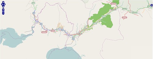
For a route I chose a GPX track I uploaded recently. There are plenty of other ways of generating a similar track: notably by using an on-line routing engine and saving the route as a GPX (for instance Open MapQuest, OpenRouteService or Cloudmade). To get the GPX track into PostGIS I used Quantum GIS to save the track as a shapefile and the SPIT extension to upload this to PostGIS. In PostGIS I added two extra geometry columns to this one row table, and updated these with the track itself and the track surrounded by a 1 km buffer:

UPDATE route_track
SET geom_goog = ST_SETSRID(ST_TRANSFORM(geom_wgs,900913),900913)
, geom_goog_buffer = ST_SETSRID(ST_BUFFER(
ST_TRANSFORM(geom_wgs,900913),1000),900913);
For each of the 4 main planet_osm_* tables I created a view as follows:
CREATE OR REPLACE VIEW planet_osm_lineX
AS
SELECT a.*
FROM planet_osm_line a
, route_track b
WHERE ST_INTERSECTS(a.way,b.geom_goog_buff)
I ran SELECT populate_geometry_columns() to ensure the geometry columns were accessible to PostGIS operations. It would be possible to rename the planet_osm_* tables and create the views instead of them. This would avoid the need to create an extra copy of the mapnik XML file, which is what I did next.

I made a copy of the mapnik.xml file and replaced all examples of planet_osm_* with the same string with an "X" appended.

All I had to do then was add a suitable bounding box to the python script and set local variables for the map tile directory & the mapnik map file. Really the bbox should be determined from the database, but the objective was to do something quick and dirty. For my example I used a bounding box which was 2 degrees wide and 1 degree high.

Tile generation runs pretty smoothly: as one might expect lots of empty tiles are created, but the query overhead is quite reasonable. As the empty tiles are only 103 bytes each they don't take up too much space either.

There are lots of fairly simple optimisations which could be added:
  • Find the bbox of the route & only generate tiles within that bbox.
  • Identify empty tiles en masse and avoid running the mapnik queries against the database for these tiles.
  • Replace empty tiles with links.


Monday 8 August 2011

Augmenting Residential Landuse : building density

Building Density on Residential polygons, Nottingham

Andy Allan (gravitystorm) asked a very pertinent question after my talk at SotMEU: Why had I not used building outlines to automatically identify different classes of residential landuse?

Briefly, my answer was: "I had tried, but the results weren't satisfactory". This is a much longer answer than I could give at Vienna, and fills in some detail about the technical approach I used. I hope that readers may have some good suggestions to improve this approach.

It is clear that Urban Atlas data is a good model for studying landuse mapping through replication/simulation in OSM. After working with this data for six months I realise that one of the main reasons for this is that UA's main classification is simpler than the current OSM consensus for landuse mapping. Thus most UA landuse classes have a 1:M mapping to OSM tags. Other landuse and landcover schemes, such as CORINE, EUNIS, have many more classes and in thus in many cases the classes have N:1 or N:M mappings to OSM tags. Most of these relate to agriculture, woodland or natural vegetation: for the most part where OSM tag usage is only fitfully consistent, or the same tag has multiple meanings.

There are, however, 5 UA classes (Continuous and Discontinuous Urban Cover — 11100, 11210,11220, 11230 and 11240) which map on to a single tag in OSM : landuse=residential. The main criterion for separating this classes in UA is the degree of surface sealing, with continuous urban cover meaning that over 80% of the land surface is effectively sealed (buildings, asphalt, concrete etc.). As a significant proportion of surface sealing will be buildings it seems plausible to use the proportion of residential landuse covered by buildings as a proxy for surface sealing.

Buildings from OSM & OS OpenData
Buildings generated from OS OpenData using mapseg (orange) compared with those mapped in OSM using Bing imagery (light green) for OS grid square SK5038.

Firstly, I needed a decent source for building outlines. My test data area, Nottingham, does have a large number of mapped buildings (47000+), but is nothing like complete. Partially mapped building sets are no use at all for this purpose. I therefore made use of Mapseg a set of python routines written by Tim Sheeman-Chase to extract building outlines from the Ordnance Survey OpenData StreetView (OSSV) tiles. I had originally created this data to make address mapping easier, but was dis-satisfied with artefacts (spiky buildings, failed orthogonalisation, etc.) so I had only used a tiny proportion of the data directly in OSM. My original data set covered the whole of the county of Nottingham and adjacent areas and included over 600000 building outlines: processing and manipulating this was somewhat tedious as each OSSV tile or sub-tile generated a single OSM XML file and I therefore had around 200 files with duplicate node and way identifiers. In the end I loaded each file into PostGIS and merged the data there. I then clipped it to the bounds of the target test area to end up with a data set of 189, 420 buildings. Some geometries needed to be cleaned to remove self-intersections.

Buildings were then clipped to match the residential landuse parcels, and then assigned to individual parcels. Landuse parcels which had originally been created as multipolygons on a 1 km grid were decomposed to individual polygons (using ST_DUMP) before this step. Polygons meeting on grid boundaries were not re-assembled. At this point it is simple to sum the building area for each polygon and determine the ratio of the total polygon area covered by buildings. The results are graphed below with the data divided into 20 buckets.

For comparison here is the relative distribution of the EEA UA data for the Nottingham area:

UA Code Area (ha) % Total Residential
11100 137 1.0%
11210 7132 52.0%
11220 5298 38.7%
11230 846 6.2%
11240 18 0.1%
11300 272 2.0%

The vast majority of residential landuse falls in two classes with surface sealing in the range 30 to 80%, with more than half of the landuse with greater than 50% surface sealing. A cursory comparison between the two sets of figures suggests that, at best building cover may only account for half factors used to assign surface sealing in Urban Atlas. Fortunately because I created a datasets of differences and similarities of data from UA and OSM it's possible to compare individual landuse polygons: a bit more work as these may be slightly different shapes, and therefore the whole clipping of buildings and area calculation must be repeated.

Comparison of UA Codes with OSM building density

The box-plot above amply confirms the initial impression. No doubt if and when I learn more about R, a proper statistical comparison could be done. Building density from OSM does not explain enough of the UA surface sealing value to be reliable for classification. At least for now. There is enough in the plot to hint that enrichment of the data with other variables may facilitate separation, but that's a different project again.

So that's the (very) long answer to Andy's question.

What does it mean for OSM:
  • Using buildings to derive sub-classes of residential landuse is not generally useful.
  • The requirement for completeness in building outlines on its own means that such an approach would at the best of times only work in certain places (good external sources of building data, excellent imagery). It may also require fanatical devotion to mapping buildings.
  • The basic classes of landuse we are interested can probably be derived from local knowledge, ground survey, aerial imagery etc. To make this more generally useful this requires some guidelines and consensus on tagging.
  • For now we could use tags similar to the Urban Atlas codes for urban areas in Europe and North America. Significant extension of these values might be needed to adequately cope with other areas in the world. (I'll be blogging in depth on this subject soon).
  • Looking at extending this type of data with other OSM derived variables may be interesting. Alexander Zipf mentioned that his group at Heidelberg had used a data mining approach to identify residential areas from OSM data.
If you've got any ideas of how to extend this type of classification drop me an email or comment below.