Mundane Cartography : mapping Vice Counties

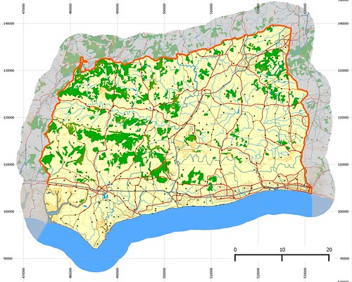
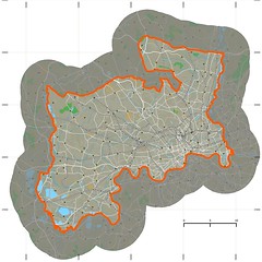
West Sussex (VC13) mapped using OS OpenData (Meridian2)
database right, Ordnance Survey, 2012

Late last year I grew increasing frustrated with the maps I use within MapMate for biological recording. Maps have two purposes: firstly they help in putting records in the right place; secondly, they provide a context for displaying cumulative sets of records (usually in a distribution atlas).

MapMate allows the creation of maps through an absolutely horrible interface. The vector sets which come with the product are too inaccurate for serious work. Long ago I moved to using geolocated images as an informational underlay within the product. I've used various techniques: grabs of OS Maps from the OS website, OSM maps generated with Kosmos or Maperitive, OS OpenData Tiles (StreetView, 250k etc). None has been wholly satisfactory: either they have too little information or too much. After several years of doing this I think I now have a much better idea of what is needed.

Typical recording focuses on small discrete areas: perhaps from 1 to 250 hectares in size. In these areas the ideal is to note precise positions of things like plants, insects and fungi, but location to within 100 metres is a reasonable compromise: the 6-figure grid reference beloved by British Naturalists. However, with one of my datasets containing well over 1000 records I noticed that using manual methods (looking at a map & assigning the record to a square) I was frequently 100 metres out. This was most noticeable with a Buckthorn growing on North Path at Attenborough Nature Reserve. There are a number of insects and fungi which are associated with this plant which I have recorded on this isolated tree. Over time I'd managed to place records in three adjacent 100m squares. Although I'm trying to move to direct data capture in the field this is still not possible in lots of circumstances. Therefore being able to create maps which have more pertinent information can help accurate recording a lot.

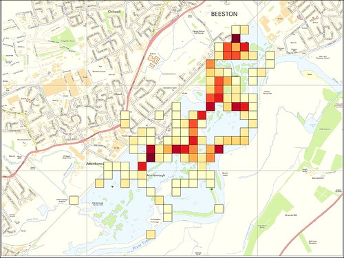OS OpenData StreetView used for recording at 100m square level

On a smaller scale the same thing happens too. For recording at the vice county level (perhaps typically 2500 km2) the currently favoured unit is the grid kilometer square or the tetrad. Again it's easy to be out by one if the map used for data entry does not have the right level of detail. I therefore wanted to create maps which I could use as a reference layer in the recording software and which had large number of visual cues to enable rapid and accurate selection of the correct grid square for recording. Obvious information includes major water bodies (lakes and rivers), larger areas of woodlands, and settlements. The road and railway network also provide useful queues. It's probably not necessary to make use of all of these, but I was interested if I could produce a simple cartographic product which could then be altered for a variety of purposes.

Long ago Richard Fairhurst had remarked that he favoured one of the OS OpenData sets, Meridian 2 or Strategi, I can't recall which, as a good base for cartography at medium scales. I'd neglected to follow this up, but recalled his argument when I started doing this. Therefore my starting point was the Meridian 2 dataset, Vice County boundaries (mean low-water line version) from NBN Gateway, and a couple of datasets showing protected areas (SSSIs and Local Nature Reserves) from Natural England.

As I wanted something fairly quick and dirty I chose Quantum GIS to do the cartography.

Firstly, I created a shapefile with the relevant vice county I was interested in, and then buffered this by 5 km to create a 'halo' to provide additional context for the map. Later I decided that I wanted to mute areas outside the county, so I created another shapefile which was the difference between the two. I achieved my goal by placing this at the top of the list of layers and making it 50% transparent.

The Meridian layers I used were, lowest layers first: Woods, Rivers, Lakes, Minor Roads, B-Roads, A-Roads, Railways, Motorways and Settlements. I added SSSI and LNR layers as hatched overlays. This produced a map which was pretty satisfactory, even though it reflects a very simple application of the Painter's Algorithm. The image below shows the QGIS workspace:

Layers showing application of Painter's Algorithm in QGIS

I've run into a few problems:

• A number of the original vice county polygons were incorrectly formed. Although it's not too difficult to identify the problem they are quite difficult to repair. Fortunately most of these are in the far north of Scotland, so don't worry me at the moment.
• OS Open Data provides the coast line as a polyline. I need land areas as polygons for various manipulations. I have therefore started creating land tiles corresponding to Ordnance Survey 100km grid squares. I am using PostGIS to do this.
• Vice County boundaries reflect mean low water tides. For areas of mud flats and sand these can be a long way from the high water line (coastline). These areas need to be split out as a distinct layer below the sea.
• Boundaries need to be changed to polylines because I don't want to show boundaries on the coast. Where two vice counties are separated by a sea channel some further work needs to be done.

I'd also like to add some more data:

• Shaded Relief
• Contours or Hypsometric tints
• Urban area landcover
• Boundaries of National Parks & Areas of Outstanding Natural Beauty (AONB)
• Parkland 
• Settlement names for larger settlements and different symbols for settlements by size.

VC49, anachronistically still called Caernarvonshire, has been my test area for some of these changes.

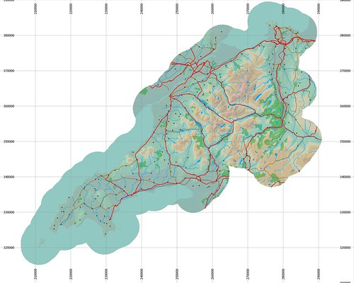VC49 Caernarvonshire with hill-shading and hypsometric tints. Note coastline issues.

Now that I have the basic idea I've got the core of the data in PostGIS. There is plenty of scope for modifying the cartography for different purposes. In particular a muted or greyscale style is desirable as an orientation layer for thematic maps. I've only just started playing with these (see below)

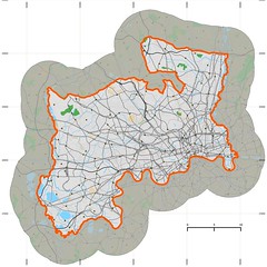VC21 Middlesex Grey on Pale

VC21 Middlesex, White on Grey

I've called this mundane cartography because there is absolutely nothing special in what I have done. I've mainly used a single dataset as is, a very simple minded version of the Painter's Algorithm, and a fairly straightforward GIS toolset.

One of the interesting things about mapping at this scale: roughly between 1:150k to 1:400k, is that there is very little data directly related to the natural landscape which it makes sense to show. Woodland, Lakes and Rivers just about covers all the areas which are likely to be useful at these scales. Natural England have a large number of datasets of special vegetation types, but many of these are barely visible even at 1:25k scales. This is particularly true now that many of these vegetation classes are much diminished in total area compared with even 50 years ago.

The reasons for not using OpenStreetMap data are very similar to those adumbrated by Richard Fairhurst: consistency, generalisation, and completeness. Mapping of woodland and water is essential for my goal: these are likely to be areas with an higher level of recording than other areas. Many large forestry areas have not been mapped, particularly in Scotland and Wales. Similarly it would have been time-consuming to try and generalise OSM data which, in the main, are too detailed for this purpose.