The reporting and discussion of a mountain rescue on the the minor Lakeland peak of Barf continues to generate a mass of things to investigate and follow-up. I've already written two OSM diary entries on assigning slope angle to paths because of it: here and here.
To recap, recently the Keswick Mountain Rescue were called out to help 3 people who were stuck ("cragfast") on steep ground on Barf. They didn't feel confident to retrace their steps back down very steep (30 degrees or over) scree and had reached a small crag with no obvious visible route through it. They had been using one of the mobile phone outdoor hiking apps which uses OpenStreetMap data for suggesting walks.
The event was reported in the national press (The Guardian) and, of most relevance, by a specialist magazine, The Great Outdoors. The latter did a great job of thoroughly researching a news article, getting comments from the OpenStreetMap Foundation. Their specialist advisor Alex Roddie decided to publish the content of his initial response to Carey Davies, the author of the article. Both articles are well worth reading for an in-depth initial response to the situation and the issues arising. There have also been lively exchanges both on Twitter and Mastodon, again containing useful comments from people with a lot of experience of the outdoor scene in the UK.
I won't comment here on the whys and wherefores of what kinds of paths and hiking routes should get mapped on OSM. The subject is complicated enough in Great Britain as all this discussion shows. One of the side distractions this did prompt for me was looking at how we could show contour data for OSM in the British Isles (and specifically on Andy Townsend's rural hiking map).
A toot by Nigel Parish did highlight that typically maps based on OpenStreetMap have contours which are greatly smoothed compared with the actual terrain. His example was from Andy Allan's Thunderforest Outdoor style which is incorporated into a number of hiking apps. Like most regular OSM contributors, I'm used to OSM-based maps using SRTM data to create contours: both because it's free and because it has more-or-less worldwide coverage. However, we are also aware of the deficiencies of this data: it has a relatively low resolution of around 1 second of arc (so roughly 30 metres resolution) which smooths contour lines and hillshade overlays.
I had recently downloaded the Ordnance Survey's own open data elevation model Terrain50, which I used for the first of my diary entries. This has a grid interval of 50 m, so although undoubtedly more accurate than SRTM, it is of somewhat lower resolution. I therefore expected contours generated from the DTM to be comparable with those of SRTM.
I'd forgotten that I'd used the vector dataset, so my first step was to generate contours from the raster tiles provided by Terrain50.
 |
| Barf with contours derived from the raster DTM of Terrain50. |
After I'd done this, I remembered that the Geopackage was easy to use, so I added that. To my surprise the contours had rather more detail than those derived from ostensibly the same dataset.

| |
Lastly, I created 10 m contours from the 1m Lidar data available from the Environment Agency for NW22NW. This, as expected shown both high resolution and accuracy.
 |
| With 10m contours derived from Environment Agency 1m Lidar. |
To compare the three types of 10 m contours I changed colours and their background. Here are all three at a scale of 1:1000 on the steep SW slope of Barf between the Bishop of Barf and the crag which balks some walkers. In the image below it can be seen that the vector Terrain50 data is of much higher resolution than the raster data from the same source. In most places vector Terrain50 data is much closer in alignment with the contours derived from 1m Lidar data. As Nigel pointed out the more detailed contours give a significantly different impression of the shape of the hillside.
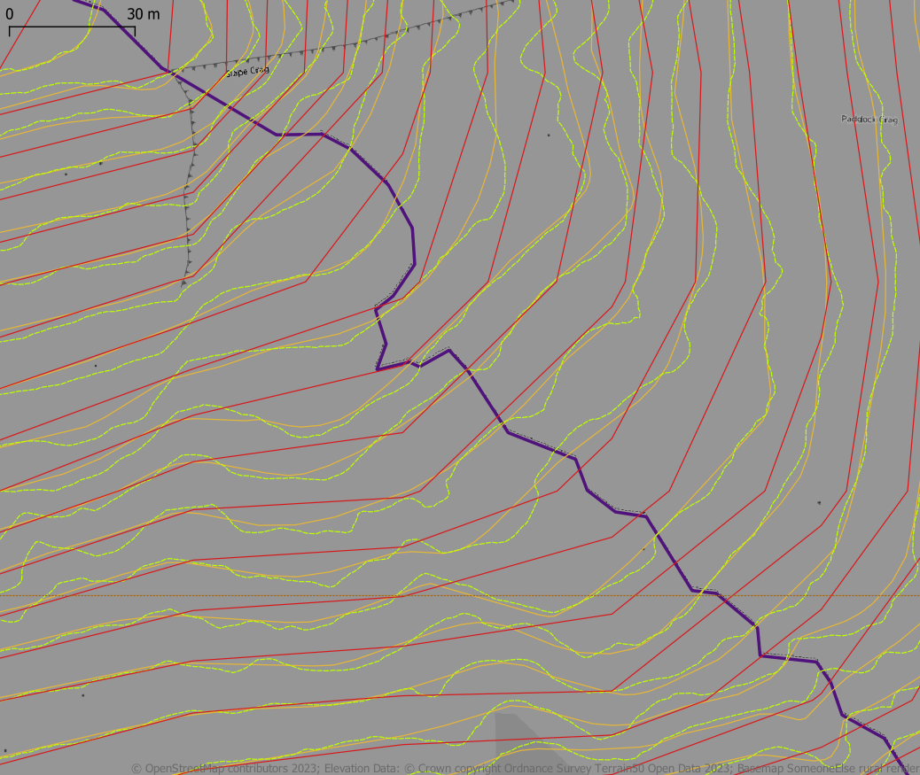 |
| All three types of contours shown together. Red derived from OS Terrain50 raster; Orange: OS Terrain50 vector; and Green derived from Environment Agency 1m Lidar DTM. Scale 1:1000. |
Nigel also pointed out that lots of relevant terrain features, shown on printed maps (Harvey & OS), and available as online tiles, were missing. This type of detail is often difficult to generate automatically using software, and even then is unlikely to match the output of skilled draughtsman working to detailed composition rules. I tried adding a hillshade layer from EA data, but it didn't really pick out this detail. Then I remembered that Luke Smith of Grough had used a layer provided with OS VectorMap District called "Ornament" when he prototyped maps based on open data. I therefore added this layer. It works quite well at low zooms, but is rather ugly at anything higher than 1:5000.
 |
| Added hillshade from Environment Agency data and Ornament from OS VectorMap District open data. Hillshade is less effective than I expected at high zooms, and the ornaments only really work in a range 1:5k (as here) to 1;25k or thereabouts. |
Lastly, and more for fun than anything else, I regenerated contours at 15 m intervals and clipped these by scree layers mapped on OpenStreetMap and changed the colour of the contours to a shade of grey to replicate how this information is shown on the Harvey Map. The end result is a good illustration of these differences: the Harvey Map generalises features such as cliffs and places them to enhance the map users' impression of the terrain, whereas the OS ornament looks nice, but is nothing like as good a guide for the walker.
 |
| With 15 m contours (from EA 1m DTM) and with contours on scree coloured grey rather than brown (as done by Harvey Maps), plus OS VMD ornament. |
The bottom line from this is quite simple: don't bother with Environment Agency Lidar data if you just want contours: Terrain50 vector data is much easier to get up and running. The data is also packaged as mbtiles, but I couldn't find a way to style this in QGIS.
Lastly a big thank you to Nigel Parrish who caused to to look at the data, and thus discover the difference between the vector & raster versions.