Another post from the past, not much map content really.
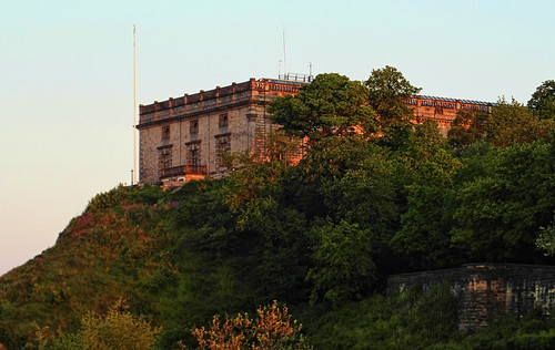
Newcomers arriving in Nottingham by train are often disappointed that the squat box perched above the railway line does not resemble their idea of Nottingham Castle. The reason why it does not look like the Hollywood image are rooted in some significant events of English history.
The Castle was the site where Charles I raised his standard at the start of the English Civil War. Victor's justice meant that the mediaeval castle was slighted (effectively demolished) soon after the end of the Civil War. In it's place the Duke of Newcastle built a
'palace ... [which] looks ... as if it stood in north Italy or Praque" (Pevsner (1979: 226), Buildings of Nottinghamshire).
In 1831 this building was burnt to a shell during the Reform Act Riots, and remained as such until 1875, when the building was restored as one of the earliest municipal museums in Britain.
I'd always known about this event, but knew little of the detail. I therefore persuaded my father to join me on a guided walk about the tumultuous days of 1831. The walk was organised by People's Histreh a group of local people interested in radical history.
We joined the group outside St. Peter's Church on the May Bank Holiday of 2011. To keep us together someone had a large loaf impaled on a stick. Apparently this was one of the codes that a riot was impending. Another signal was to grab whole cheeses off market stalls and roll them in the street. (Nottingham had a "Great Cheese Riot" in 1766).
The route followed is shown above. Abbreviated audio of the talks given can be found here and here on Youtube. The embedded video gives feel for what the walk was like, with the early part of the talk by Phillip,an excellent guide.
One of the advantages of failing to finish writing blog posts is that one event overtakes another. In August 2011, Nottingham, like many other English towns, had sporadic events of rioting. At the time I mapped the locations of people brought before the courts for offences connected with rioting:
I'm not sure that any specific lessons can be learned from this plot: locations of riot damage might make it more informative. Unfortunately I don't have either the data or a useful map of 1831 to do something equivalent for the Reform Act Riot.
My impression is that people had travelled quite a distance from their home addresses to the places where riotous events took place. Earlier riots in Nottingham, such as those of 1981 in Hyson Green were much more localised.
In the area of Zurich where I used to live (Kreis 4, Aussersihl) it is still traditional to have a riot every 1st of May. Sensible people get out of town.
and another:
The 2011 riots in England were seen as an exceptional event motivated by "sheer criminality". However, any serious consideration of riots must take them as a recurrent feature of any urban environment: whether they be motivated by poverty, political unrest, or the dynamics of crowds.
Changes:
Jan 2016: replaced Geocommons embedded map with same data moved to Umap.
Before SOTM-EU 2011 I wanted to spend a bit of time in the Alps. This is a belated account of that trip.
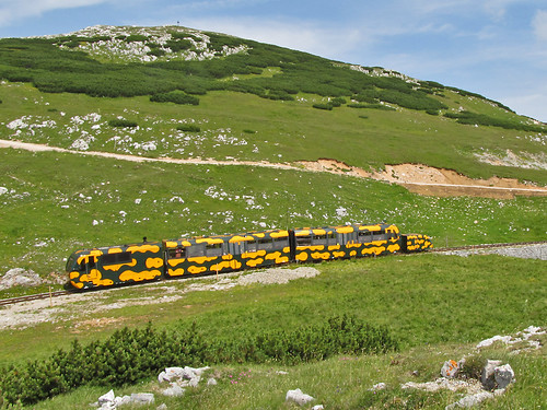
Salamanderzug near the top station.
It's been a few years since I've been anywhere in the Alps in Summer, and in the meantime I've improved my botanical knowledge enormously. So high on my list of things to do was to look at alpine flowers properly for the first time. This is pretty much incompatible with serious hiking: botanising takes time, it's eminently possible to travel at about 100 metres/hour.
I therefore wanted somewhere close to Vienna with mountains high enough to have an alpine flora still in flower, and some kind of mechanical uplift. The obvious choice was the Wiener Hausgebirge, groups of limestone peaks reaching over 2000 m about 50 km SW of Vienna I've known about this area for a number of years: when my brother lived in the Viennese suburb of Meidling, I went skiing on a local hill, the Zauberberg at Semmering. At that time I noted the peaks of the Rax-Schneeberg area from the wonderful switchback railway over the Semmering pass.
The village of Puchberg-am-Schneeberg is still a popular day-trip destination from Vienna, but in the past was a small spa resort. There's one large hotel and a smattering of smaller places. I stayed in the Bruckerhof which turned out to be a nice place in a good location at a great price. It is only a couple of hundred metres from the station, and set back from the main road.
Puchberg was pretty quiet in the evening. I had the impression most visitors were, like the guests in my hotel, of a certain age. I was troubled that I'd have difficulty finding a place to eat, as most people seemed to have dined by half-past six. However, the Schwarzer Adler not only did food, put had a proper pub-like atmosphere down to guys playing cards at the Stammtisch.
With an altitude range of around 1500 metres from the village at just under 600 m to the summit of the Klosterwappen on the Schneeberg at 2076m there was a huge range of interesting habitats to explore. The only downside was that most of the lowland hay meadows had just been cut: so I missed out on some obvious places to botanise. On my first afternoon I wandered (very slowly) up the zigzag track through pine woods to the little peak of the Himberg.
Edelweiss (Leopondtidum nivale)
The following morning I caught the Salamanderzug up the mountain. Even from the train there were special (and protected) flowers to be seen: Martagon Lily Lilium martagon (Türkenbund), Nottingham Catchfly Silene nutans (Nickendes Leimkraut), and Carthusian Pink Dianthus carthusianorum (Kartäusernelke). On the plateau the highlight was Edelweiss (Leontopondtium nivale) and masses of Mountain Avens Dryas octopetala (Silberwurzen). The latter gives its names to stages of the post-glacial Quaternary, so it's more than a pretty flower.
What has this to do with maps? Well the whole area around Puchberg and the Schneeberg itself are great exemplars of the sort of habitats (strictly biotopes) of the kind I would like to map.
Walking up the path to Himberg, I started in woodland dominated by Austrian Pine (Pinus nigra ssp., Schwarzkiefer), but on the northern side of the hill, this graded in Spruce Picea alba woodland (Tannenwald). Further along there were areas of Beech woodland (Buchenwälder). These are very noticeable: the pine wood has much more light than the spruce wood, and very different plants in the under-storey. Beech woods are different again. The plateau of the Schneeberg was a mosaic of grazed areas with a wide range of herbs and sub-shrubs (Mountain Willows, Mountain Avens, Dryas octopetala; Rose), and extensive areas of Pinus mugo scrub. These can be seen behind the train in the picture at the head of this entry. On the steeper sides of the Schneeberg, flushed areas within the Pinus mugo scrub had different plants again, such as Water Avens and . These were frequented by Fritillary butterflies. The scrub grades into forest, but at around 1000 metres there were many hay meadows, again with a different flora: it was around that I saw Martagon Lily.
The Schneeberg is also an important water catchment area for Vienna. There are a number of limestone sink holes in the summit area from which the general public is excluded to avoid polluting the supply. Again this is a feature which is still difficult to map in OSM.
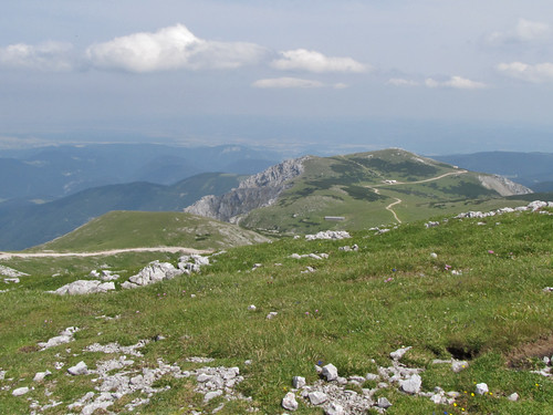
From near Klosterwappen looking across Ochsenboden
The official map made by BEV doesn't do a bad job of showing some of this information, despite really being a 1:50k topomap. It has a lot of toponymic detail, maps the Pinus mugo scrub, shows a lot of detail of the NE-face. It doesn't attempt to separate out the different forest biotopes: this is something I think is an eminently practical thing to do in OSM. The Schneeberg area is a great place to start.
Another aspect of the Schneeberg is that the NE face offers fantastic opportunities for spring skiing. I discussed this briefly with Felix Hartmann (extremecarver) after SotM-EU, who knows this area well. These are extremely well known, but not mapped on OSM. We don't have a sensible way to map this kind of ski route, nor for labelling features such as chutes, couloirs and gullies.
Ash Dieback is a tree disease which has been affecting European trees for over a decade. It hit the news in Britain when it was detected in many places last Autumn.
As this is a blog about maps, I won't dwell on the supine official response to this disease as a threat or once I arrived. Peter Marren guesting on Mark Avery's blog covers the important ground.
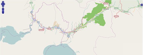
What struck me was this map in the Economist in an article about the disease (I'm not the first to use the Ashes to Ashes line from the Book of Common Prayer). It's quite a nice map, lots of information, pleasant muted colours etc. Unfortunately it's complete bollocks as a map of the distribution of Ash trees.
The clue lies in the the oddly shaped blank area near the border of Wales. I instantly recognised the shape of the traditional/historical county of Worcestershire. It is extremely unlikely that Ash trees exist in all the surrounding counties but not in Worcestershire. So it's unlikely the map is right.
There are some other suspiciously blank areas including Nottinghamshire (which would be a surprise to Neil Pinder), and an area North of London which actually has a disease record. So what's going on?
I had only to look at the map to know where The Economist sourced it's data, because there is only one source where data exists for some counties and not others. This is the Botanical Society of the British Isles online research database. To quote "Because this is research-level, live data it may not be appropriate for the general public or for consultancies." And that, The Economist, includes you.
The BSBI Distribution database is used by BSBI recorders who are organised at the county (strictly vice-county) level. They can add their data to the central database or not. Obviously the recorders for vice counties 20 (Hertfordshire), 37 (Worcestershire) and 56 (Nottinghamshire) have not added their recent data. Other places in Scotland and Ireland don't have many botanists: indeed the official recorder for the Outer Hebrides lives in South Wales, and that for Mull in Cambridge. So the map above is more accurately a map of BSBI recorders and their technology preferences. Not the best map to choose.
It gets worse. The public face of the database allows two options: distribution mapped at 10km squares (such as SK53) or 2km squares (called tetrads in Britain). The 10km square distribution data is not as up-to-date but is much more robust because it includes all records used in the major published atlases of British plants: The Plant Atlas and The New Plant Atlas. Here is what the distribution of Ash looks like at the 10km square level:
Ash distribution by 10km square (BSBI)
This shows that Ash is ubiquitous with the minor exceptions of Shetland, parts of the Outer Hebrides and the far North of Scotland.
If we look at the tetrad data including the default date partitioning, not only are the gaps obvious, but also the way the datasets for individual vice counties have been loaded at different times. For instance data for Oxfordshire are there, but are of rather antique. Thus the tetrad maps tell us far more about the internal processes of plant distribution mapping by the BSBI, than they do about Ash trees. (This is a common problem with most biological recording: the maps show where mappers are not where insects or plants or fungi might be found).
In order to display the data in a way closer to the original map from The Economist I've shown the data without date class partitions in the lower of these two maps:
Given equal access to the two datasets the creator of the graphic in The Economist clearly chose the one which looked prettier (FSVO...), rather than the one which was accurate. This is probably symptomatic of the ash dieback disease as a whole, with government bodies (Forestry Commission, DEFRA, etc.) all preferring the wind-blown arrival hypothesis over the importation hypothesis. The former is much more convenient to let the official bodies off the hook: but there is only circumstantial evidence in its favour. The alternative that the disease arrived in imported plants has a substantial material evidence base. Occams' Razor anyone?
I came into England with Oak, Ash and
Thorn, and when Oak, Ash and Thorn are gone I shall go too.
Rudyard Kipling, Weland's Sword from Puck of Pook's Hill
Gordonjcp was wanting to have a set of offline tiles for his 'phone along a route he is taking tomorrow. The ability to create a limited set of tiles would get round some of the problems associated with tile scraping, limited storage space, and time taken to create the tiles.
However, there aren't any obvious apps which do this. It occurred to me that it might be possible to limit this on the SQL side with little or no change to the standard generate_tiles.py script which is distributed with the OpenStreetMap mapnik renderer.
The idea was so simple it was worth trying out. I already had a PostGIS database containing (fairly) recent data for Great Britain, so all I had to do was import a route into the same database and create views which limited the OSM data to areas adjacent to the route. This is a very simple-minded hack, but it seems to work reasonably well and it may be possible to improve it by adding a little code to the existing python script.
For a route I chose a GPX track I uploaded recently. There are plenty of other ways of generating a similar track: notably by using an on-line routing engine and saving the route as a GPX (for instance Open MapQuest, OpenRouteService or Cloudmade). To get the GPX track into PostGIS I used Quantum GIS to save the track as a shapefile and the SPIT extension to upload this to PostGIS. In PostGIS I added two extra geometry columns to this one row table, and updated these with the track itself and the track surrounded by a 1 km buffer:
For each of the 4 main planet_osm_* tables I created a view as follows:
CREATE OR REPLACE VIEW planet_osm_lineX
AS
SELECT a.*
FROM planet_osm_line a
, route_track b
WHERE ST_INTERSECTS(a.way,b.geom_goog_buff)
I ran SELECT populate_geometry_columns() to ensure the geometry columns were accessible to PostGIS operations. It would be possible to rename the planet_osm_* tables and create the views instead of them. This would avoid the need to create an extra copy of the mapnik XML file, which is what I did next.
I made a copy of the mapnik.xml file and replaced all examples of planet_osm_* with the same string with an "X" appended.
All I had to do then was add a suitable bounding box to the python script and set local variables for the map tile directory & the mapnik map file. Really the bbox should be determined from the database, but the objective was to do something quick and dirty. For my example I used a bounding box which was 2 degrees wide and 1 degree high.
Tile generation runs pretty smoothly: as one might expect lots of empty tiles are created, but the query overhead is quite reasonable. As the empty tiles are only 103 bytes each they don't take up too much space either.
There are lots of fairly simple optimisations which could be added:
Find the bbox of the route & only generate tiles within that bbox.
Identify empty tiles en masse and avoid running the mapnik queries against the database for these tiles.
Andy Allan (gravitystorm) asked a very pertinent question after my talk at SotMEU: Why had I not used building outlines to automatically identify different classes of residential landuse?
Briefly, my answer was: "I had tried, but the results weren't satisfactory". This is a much longer answer than I could give at Vienna, and fills in some detail about the technical approach I used. I hope that readers may have some good suggestions to improve this approach.
It is clear that Urban Atlas data is a good model for studying landuse mapping through replication/simulation in OSM. After working with this data for six months I realise that one of the main reasons for this is that UA's main classification is simpler than the current OSM consensus for landuse mapping. Thus most UA landuse classes have a 1:M mapping to OSM tags. Other landuse and landcover schemes, such as CORINE, EUNIS, have many more classes and in thus in many cases the classes have N:1 or N:M mappings to OSM tags. Most of these relate to agriculture, woodland or natural vegetation: for the most part where OSM tag usage is only fitfully consistent, or the same tag has multiple meanings.
There are, however, 5 UA classes (Continuous and Discontinuous Urban Cover — 11100, 11210,11220, 11230 and 11240) which map on to a single tag in OSM : landuse=residential. The main criterion for separating this classes in UA is the degree of surface sealing, with continuous urban cover meaning that over 80% of the land surface is effectively sealed (buildings, asphalt, concrete etc.). As a significant proportion of surface sealing will be buildings it seems plausible to use the proportion of residential landuse covered by buildings as a proxy for surface sealing.
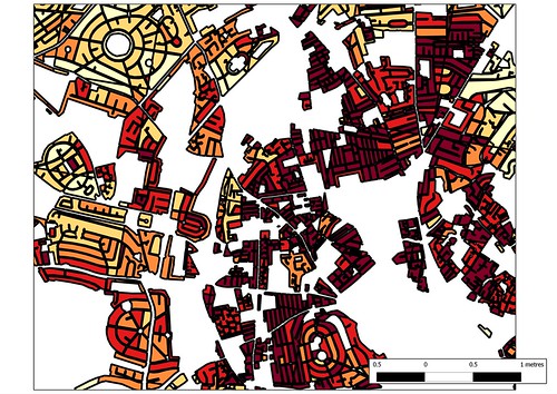
Buildings generated from OS OpenData using mapseg (orange) compared with those mapped in OSM using Bing imagery (light green) for OS grid square SK5038.
Firstly, I needed a decent source for building outlines. My test data area, Nottingham, does have a large number of mapped buildings (47000+), but is nothing like complete. Partially mapped building sets are no use at all for this purpose. I therefore made use of Mapseg a set of python routines written by Tim Sheeman-Chase to extract building outlines from the Ordnance Survey OpenData StreetView (OSSV) tiles. I had originally created this data to make address mapping easier, but was dis-satisfied with artefacts (spiky buildings, failed orthogonalisation, etc.) so I had only used a tiny proportion of the data directly in OSM. My original data set covered the whole of the county of Nottingham and adjacent areas and included over 600000 building outlines: processing and manipulating this was somewhat tedious as each OSSV tile or sub-tile generated a single OSM XML file and I therefore had around 200 files with duplicate node and way identifiers. In the end I loaded each file into PostGIS and merged the data there. I then clipped it to the bounds of the target test area to end up with a data set of 189, 420 buildings. Some geometries needed to be cleaned to remove self-intersections.
Buildings were then clipped to match the residential landuse parcels, and then assigned to individual parcels. Landuse parcels which had originally been created as multipolygons on a 1 km grid were decomposed to individual polygons (using ST_DUMP) before this step. Polygons meeting on grid boundaries were not re-assembled. At this point it is simple to sum the building area for each polygon and determine the ratio of the total polygon area covered by buildings. The results are graphed below with the data divided into 20 buckets.
For comparison here is the relative distribution of the EEA UA data for the Nottingham area:
UA Code
Area (ha)
% Total Residential
11100
137
1.0%
11210
7132
52.0%
11220
5298
38.7%
11230
846
6.2%
11240
18
0.1%
11300
272
2.0%
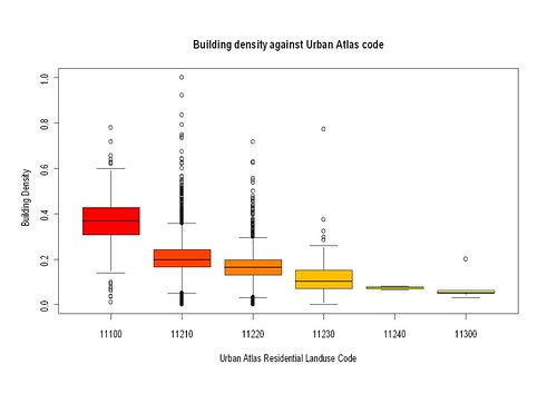
The vast majority of residential landuse falls in two classes with surface sealing in the range 30 to 80%, with more than half of the landuse with greater than 50% surface sealing. A cursory comparison between the two sets of figures suggests that, at best building cover may only account for half factors used to assign surface sealing in Urban Atlas. Fortunately because I created a datasets of differences and similarities of data from UA and OSM it's possible to compare individual landuse polygons: a bit more work as these may be slightly different shapes, and therefore the whole clipping of buildings and area calculation must be repeated.
The box-plot above amply confirms the initial impression. No doubt if and when I learn more about R, a proper statistical comparison could be done. Building density from OSM does not explain enough of the UA surface sealing value to be reliable for classification. At least for now. There is enough in the plot to hint that enrichment of the data with other variables may facilitate separation, but that's a different project again.
So that's the (very) long answer to Andy's question.
What does it mean for OSM:
Using buildings to derive sub-classes of residential landuse is not generally useful.
The requirement for completeness in building outlines on its own means that such an approach would at the best of times only work in certain places (good external sources of building data, excellent imagery). It may also require fanatical devotion to mapping buildings.
The basic classes of landuse we are interested can probably be derived from local knowledge, ground survey, aerial imagery etc. To make this more generally useful this requires some guidelines and consensus on tagging.
For now we could use tags similar to the Urban Atlas codes for urban areas in Europe and North America. Significant extension of these values might be needed to adequately cope with other areas in the world. (I'll be blogging in depth on this subject soon).
Looking at extending this type of data with other OSM derived variables may be interesting. Alexander Zipf mentioned that his group at Heidelberg had used a data mining approach to identify residential areas from OSM data.
If you've got any ideas of how to extend this type of classification drop me an email or comment below.
This is a very belated write-up of the May Nottingham pub meet-up.
First of all it was great to meet will_p, our most productive local mapper, and to welcome Paul the Archivist who has mapped actively in his home town Derby, Birmingham and Cardiff. A few of us met at the pub for an hour walk and a bit of light mapping: this is always a good opportunity to compare notes about how different people map and talk about specific issues as they arise (such as how does one represent the surface of the road below: we didn't have a good answer!).
I find it difficult to think of an area comparable to that around the Lincolnshire Poacher which has a similar variety of different sorts of places within a couple of hundred metres: modern social housing, schools, a university campus, retail and commercial areas, pre 20th century housing, large houses, parks, gardens etc. It's also not that well-mapped, something which only really becomes apparent by walking through and checking OSM with what's on the ground. In fact our little mapping walk showed, once again, how much can be missed when one only uses aerial imagery.
We again chased down a few missing road names, but failed to see any signs on one road. Marcus pointed out a few streets along Woodthorpe Road which were blocked and not mapped properly (these are tree-lined so guessing that they connected from aerial imagery was wrong).
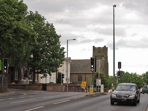
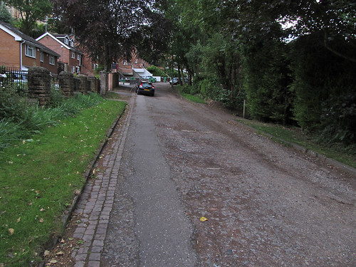
This time we headed into the S edge of Mapperley Park, one of the wealthier parts of the city, and a great contrast from St Anns, just the other side of the ridge line. We only followed three or four roads but it was very clear that the original sources of OSM data were pretty poor: this was a mix of NPE maps and aerial imagery. Density of mature trees in Mapperley Park made it difficult to identify the actual road lines from aerial imagery. We walked down Redcliffe Road the upper parts deeply cut into the rock and supported by Bulwell Stone walls . These stone walls area a classic sign locally of a private development between about 1880 and 1960. After 1960 the quarries were running short of this attractive Magnesian Limestone. Many are now used for housing or industry close to Bulwell town centre.
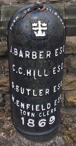
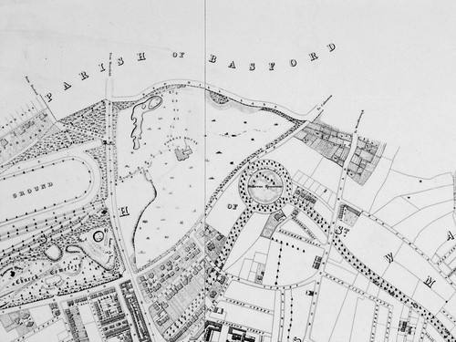
The most interesting site along this road were a couple of cast-iron boundary markers from 1859: these list the mayor and town clerk of the Town of Nottingham (it didn't become a city until some time later). In style they are very similar to the markers used when the City boundaries were extended in the 1930s (see an earlier post). I was intrigued because I didn't know which area was on the other side of the boundary. Fortunately we have an old map at home (Salmon's map) which is virtually contemporaneous with these boundary markers. I took a couple of pictures of the same area that we walked through showing the state of Nottingham in the early 1860s. This clearly shows the boundary, and that Mapperley Park and much of the Forest were in the parish of Basford. Basford was incorporated into Nottingham in the 1880s.
Also of interest is that the road was then called Red Hill Lane. Some road names in St Anns have been preserved although in altered form after re-development, but quite a few on the roads around Bellevue Reservoir seem to have been lost. It's not clear what name the paths round the reservoir have themselves: this old map calls it St. Anns Hill, which now belongs to a road which was then called Blenheim Villas, whereas modern maps (and some from the 1930s) name it as part of Corporation Oaks.
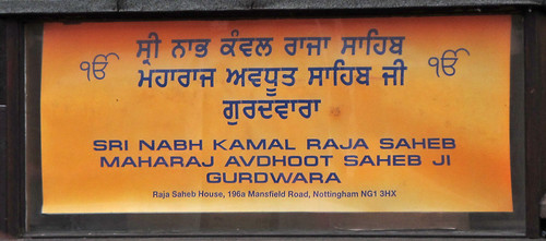
Returning to the pub along Mansfield Road we had a better look at the prominent church shown at the top of the blog. Paul had noted that it seemed to be a Gurdwara, a Sikh Temple, and as we passed it took a 'photo of the notice board. The following day I felt compelled to do a bit of research: How long had it been a Gurdwara? Who built it? what was it's recent history? I was relieved to discover that it had recently been acquired from the Christian Scientists who have moved their place of worship into their fine office building next door. But originally it was built as a Presbyterian church. So it had been a church when first mapped on OSM, but another object lesson that things ain't what they seem and the importance of ground surveys.
We ended up in the snug at the Poacher for a pie (Paul) and several pints.
SK53 received a Garmin GPS as a Christmas present in 2008. Foolishly he downloaded OSM, noticed a nearby street was missing, and promptly sold his soul to mapping. Since then he has mapped large parts of Nottingham, verified about half of Maidenhead, takes a PC on holidays for mapping, and now has 2 more GPS gadgets, but still feels the need for more. Further details on his OSM wiki page User:SK53