Urban Areas 2 : Derivation from OpenStreetMap using Residential Roads

Street corner, Retiro, Buenos Aires
(Libertad/ Juncal)
CC-BY-SA, the author

Following on from my last post I have now been looking in more detail at how one might start using OpenStreetMap (OSM) to create a global dataset of Urban Areas. As OSM does not have any widely used notation for urban areas I have been looking at several ways in which other OSM data can be used to identify such areas prospectively. In this post I look at the use of residential roads (and I'm not the first to do so). Later posts will look at other techniques.

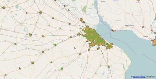Buenos Aires and hinterland, showing comparison between urban polygons
derived from OSM (green) and the Natural Earth data (light brown).

I have chosen the following places as suitable test areas for these investigations:

• East Midlands of England. Not only my home turf, but also a well-mapped area with extensive use of landuse tags, and in excess of 99% of all residential roads. In addition Ordnance Survey Meridian 2 Open Data contains a layer corresponding to urban areas which provides an excellent control for checking results from this area.
• Pakistan. Not only one of the most populous countries in the world, but one of the least well mapped in OpenStreetMap. Pakistan is a likely candidate for cities which are barely mapped. I would also expect other very populous Asian countries (notably China, India and Bangladesh) which are poorly mapped to be similar to Pakistan.
• Nigeria. Similar criteria to Pakistan: the most populous country in Africa. The .pbf file for Nigeria is approximately 50% larger than that for Pakistan, but both are smaller than that for Lesotho with a population of 2 million compared to 180 million (Nigeria) and 200 million (Pakistan).
• Côte d'Ivoire. Close to Nigeria, but a place which I know has an active OSM community. Quite a number of mapping activities. (Note to Geofabrik, it's not called the Ivory Coast any more).
• Argentina. Latin American cities are often laid out in a grid, nowhere more so than in Argentina. The prevalence of the grid system, and my believe that the urban road system is largely complete were reasons for choosing this as a Latin American example. My own experience of travelling in Argentina after SotM-14 suggests that, for the most part, urban road systems are mapped. One known gap, the newer western suburbs of Ushuaia has recently been rectified by the kind provision of aerial imagery from the Argentine National mapping agency.
• Pennsylvania. It was essential to include some US data  because of the TIGER import problem: all rural roads being tagged residential. Since I spent part of my childhood in Pennsylvania it is also a place I know and which I have edited (sporadically) to improve the rural road network.

Briefly I expected the following: good urban areas for the East Midlands and Argentina (i.e., better than Natural Earth (NE)); middling to poor for the three developing nations (gaps relative to NE, but in some cases better precision); hopeless for Pennsylvania.

The basic process is very simple:

1. Extract residential roads
2. Merge all roads which link together into a single multiline segment
3. Buffer each group of merged roads (I use 100 metres)
4. Buffer again by a larger amount & then again by the same amount but negated: this smooths the outline and fills any residual holes.

In practice this needs to be slightly more complex to improve performance. To this end I add the following techniques:

•  Roads are clipped into grid squares (typically 10 km, 3 minutes or 7.5 minutes).
• Merging is first performed within the grid
• Some tidying up of this data is then done, notably buffering and re-clipping to the grid
• A second round of merging is performed ignoring the grid

I'm using the postgres routine I described a couple of years ago to identify the independent graphs of roads in each grid, and in the second step. It still lacks all the performance optimisation stuff I meant to do back then! (After much messing about it turned out that it only needed indexes on the work table).

East Midlands

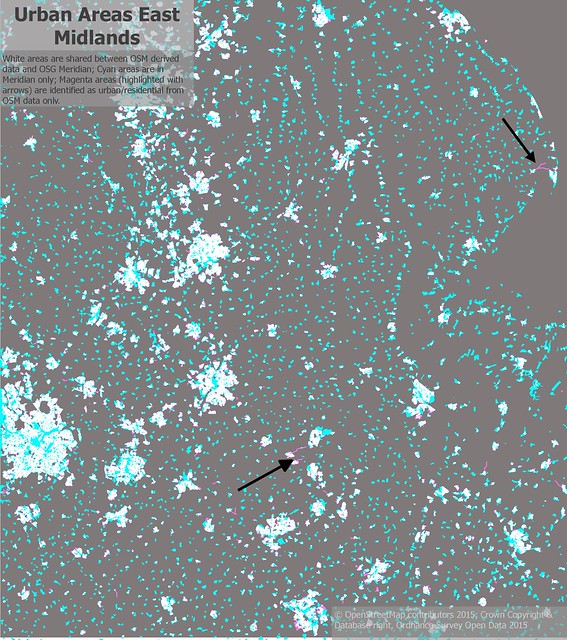Comparison of Urban Areas for English East Midlands

As expected, there is a high degree of concordance between areas identified as urban from the OSM residential road data, and the available Open Data from the Ordnance Survey. Areas not identified as urban from the OSM data, but so identified as such in the Meridian data are shown in cyan in the map above. For the most part the differences fall into two classes:

1. Commercial, retail & industrial areas in towns and cities which are not identified through merely looking at residential roads in OSM. This initial aspect of the data is of course wholly predictable.
2. Small towns and villages in the countryside. Firstly, the goal is not to find these in these experiments. Various refinements (such as adding isolated island residential roads back at various steps in the process) have not been made (see further below). Secondly many villages will be aligned along road classes other than residential and would not be found anyway. Most of these areas not identified are under 60 ha in size.

More surprising is the very small number of false positives in the data derived from OSM. These are all erroneous classifications of rural roads as residential ones (sometimes because the same road starts in a town and runs into the countryside). For Britain, at least, this offers a useful visual QA tool for OSM data.

Argentina

I had also chosen Argentina as an area to validate the concept.  But this was also influenced by the particular problems with Natural Earth data in this region. The huge megalopolis of Buenos Aires was also useful for making sure the chosen algorithms of this technique will work with the largest cities in the world.

Northern Santa Cruz & S. Chubut provinces, Patagonia
comparison of NE & derived OSM data.

Once again there is a highly satisfactory match with Natural Earth data around Buenos Aires. In Patagonia, not only are many cities which were missed by Natural Earth identified, but there do not seem to be any obvious false positives. Indeed with some light tidying-up (clipping to coastlines, filling small holes, some smoothing) this could make a viable replacement for the NE data here.

Neuquén city (bottom centre) and province: More false positive Urban Areas from Natural Earth compared to OSM
Sources: as before

Addendum

It turns out that I'm not the first to use this approach in Argentina. After I'd published this post
Nicolás Álvarez drew my attention to a talk, which I had missed, at State of the Map 2014 in Buenos Aires. The authors are :Vladimiro Bellini, Fernando Pino, Martin Moroni of the Ministry of Energy. Another great example of how people are doing interesting things with OSM data all over the world.

I haven't looked at the details yet, but from the abstract this looks very similar to my approach with an important refinement, restricting the length of roads included to those under 2 km. Slides of this talk are available on Slideshare.

Pakistan

Punjab area of Pakistan: comparison with Natural Earth.
Lahore is bottom right & Rawalpindi top left.

A first cursory look at the results for Pakistan compared with Natural Earth data suggests that most major urban areas are being detected. Looking at a larger scale reveals many mid-size cities being ignored. At even larger scales the inaccuracy of the Natural Earth data itself becomes more apparent.

Slightly more detail with Lahore (bottom centre) & Sialkot (centre).
Many rural as well as urban roads have the residential tag in the latter area,
Note the reticulated appearance of the polygon (see below, Pennsylvania)

It seems that a significant problem exists with my algorithm for Pakistan. Even large cities may have only a handful of roads mapped as highway=residential. These either form isolated islands in the first phase or are merged into a single island after the first phase. At present I make no attempt to add back these polygons with no adjacent ones. The sensible place to do it is after the second phase of merging. To do it earlier would be to introduce too many artefacts from inappropriately tagged roads or isolated residential districts in rural areas. I have not done this for this post, but show below the difference between 1st phase (dark blue) & 2nd phase (light blue) urban polygons above & below.

Higher zoom of area West of  Sialkot (right).
Many urban areas have either a tiny number of residential roads or none at all.
Source: Natural Earth & derived OSM polygons
Background Imagery: Landsat via Bing Maps

Lahore is is a megalopolis, but it has remarkably few residential streets mapped. A major factor is that in the older parts of the city, most thoroughfares in residential areas are narrow, and lined by multi-storey buildings. This makes them more or less impossible to pick out on available aerial imagery, and perhaps on any imagery likely to be available to OSM in the near future. However, my choice of buffer size to build residential roads works reasonably well even when the grid is partially mapped, as in this case.

Notwithstanding this there are still many wider roads which can be mapped. Once again I have spent a little time whilst writing this post adding a few in Lahore.

A busy street, Sialkot 2008
CC-BY-SA via Wikimedia

Elsewhere, a local mapper in Sialkot has been adding this type of detail, but using the tag highway=service, service=alley. This seems an entirely reasonable choice of tags: if it is a local convention then taking account of this by adding such ways to the choice of residential roads is easy to do. (I would have to look at the use of this tag combination globally to see if there were any problems in doing this by default).

Pakistan showing both Urban & OSM Residential areas.
Note the density in Sindh, the result of a HOT activation

It was no surprise that OSM data for Pakistan are incomplete in many areas. I have drawn most of my examples from a particularly densely populated parts of the Punjab. In the process of examining the area it is clear that much can be achieved in a relatively short time by adding more residential areas and prominent residential roads. We should bear in mind that the dreadful flooding events of 2010 are unlikely to be isolated events. At the time map data available to relief organisations was poor, and the sheer extent of the area covered was far too large for a responsive mapping campaign.

OSM data for Pakistan is still poor over 5 years on, we never managed to achieve the same leverage as Google Map Maker with the diaspora of people with Pakistani-heritage. But we can try again.

Nigeria

Roundabout Ibadan
Whilst looking for CC-BY-SA images for urban areas of Nigeria I noticed a few shots of roundabouts with distinctive sculptures in the middle. These seem quite common across the country.
Source: Adebisi Adewoyin via Wikimedia Commons CC-BY-SA

In many ways the situation in Nigeria is similar to Pakistan: at an overall level the results look reasonable, a closer look reveals that large cities are getting missed. This is most noticeable in the Southern part of the country.

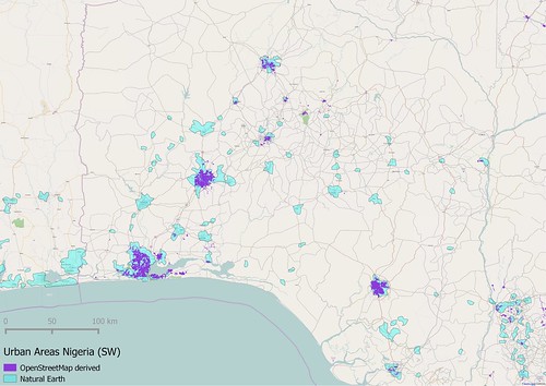Comparison of Natural Earth & derived OSM Urban Areas for SW Nigeria

For the area shown above at least one factor is the absence of high resolution imagery. However, some significant cities were missing in any other form than an imported GNIS node ( e.g., Owu). Looking at the country as a whole, it appears the North is much better mapped, with a more extensive road system and lots of minor settlements mapped as residential areas.

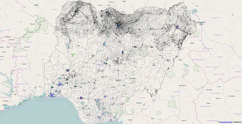Urban (NE & derived OSM) and residential areas in Nigeria

I have no idea why this should be, but clearly one would expect as much or more detail in other parts of the country based on available demographic data (see below). I am aware that Kano seems to have the most active mappers, that there have been HOT initiatives in NE Nigeria, and that eHealth Africa have been doing some mapping of residential areas (see this recent blog post): it is probably the latter activity which has had the biggest effect. I dont know quite how long this has been running, but it does demonstrate how much data can be added.

Nigeria Population Density, 2000
Compare with density of residential mapping on OSM
Source: see map CC-BY-SA

Côte d'Ivoire

Central Abidjan, quartier Plateau (on OSM)
Source: Zenman via Wikimedia Commons

I wanted to look at an area with some similarities to Nigeria, but with a better established mapping community to see if this makes for any significant difference. The obvious choice was Côte d'Ivoire. There always seems to be something interesting going on there: mapping parties, software training events, conferences. And it's all nicely documented on the community website. One of the things I particularly like is a map of pharmacies in Abidjan on umap: a reminder that maps help everywhere for little daily tasks or personal emergencies. Looking at Pascal Neis' maps Abidjan looks to be the place with the most dedicated mappers.

Comparison of NE & derived OSM Urban Areas, Southern Côte d'Ivoire
Legend: road network (OSM), NE urban (cyan), OSM derived urban (magenta)
Imagery: Landsat via Bing Maps

Again on the small scale we have a pattern of significant settlements being captured from OSM and some smaller places being missed in a fairly haphazard way. We also get the impression that NE urban areas are frequently too large.

Comparison of NE & derived OSM Urban Areas, Southern Côte d'Ivoire
Legend: road network (OSM), NE urban (cyan), OSM derived urban (magenta), OSM residential (blue)
Imagery: Landsat via Bing Maps

This is confirmed by zooming in.

Adding an extra layer from OSM, mapped residential landuse shows what is most different between Nigeria & the Côte d'Ivoire. Individual settlements of different sizes have been mapped in the latter as landuse=residential, even if no-one has had time to add the individual roads. In Côte d'Ivoire it is detail of settlements that is missing not settlements themselves.

Comparison of NE & derived OSM Urban Areas, Abidjan
Legend: road network (OSM), NE urban (cyan), OSM derived urban (magenta)
Imagery: Standard OSM layer

Looking at Abidjan itself, we can see how well mapped it is, the precise correspondence of derived urban areas with landuse mapping, and, once again, that the NE polygon is too large. I do note that the derived urban area includes some large industrial landuse polygons. This suggests that highway=residential has been used rather than highway=unclassified in these areas.

Unlike Nigeria & Pakistan (and the US, see below), I have not felt the need edit OSM for Côte d'Ivoire, either to add really obviously missing data, or to modify tagging.

Looking at these three countries together, the key point is that, unless the local OSM community is large, and mature, residential roads will not be adequate on their own to identify urban areas. In Britain, it was not until after we had official open data (Ordnance Survey) that many residential roads were added, and that was in 2010, 5 years into mapping the country. Without that external source we would probably still have significant towns & cities only partially mapped. Much of how the map  Côte d'Ivoire looks now is very reminiscent of Great Britain before we had open data: great detail in places, but fairly scanty away from where most mappers lived.

Adding landuse is an excellent way to build up a picture of what needs to be mapped: in places like Côte d'Ivoire the combination of using both landuse & derived urban areas looks promising (more later).

Pennsylvania (and elsewhere in US)

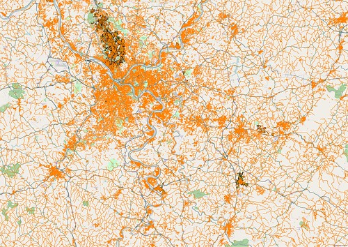Pittsburgh area : Residential Highways & Landuse mapped on OpenStreetMap
Source: (c) OpenStreetMap contributors

A quick look at road data for Pennsylvania shows that the network of residential roads reaches into the furthermost reaches of the state. The human eye can quickly discern the much greater density of the road network which represents truly urban locations. Finding a suitable automatic substitute will be the topic of a later post in this series.

However, the reason for looking at the US was to look at the problem where residential roads have not been distinguished from other minor roads (i.e., the confusingly named "unclassified" highway tag in OSM). The first thing is just to take a look at the output from the algorithm described above.

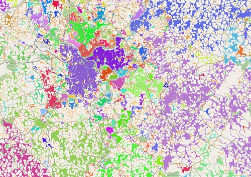The same area as above, with each contiguous group of residential roads given a random colour.

Actually it's not quite as bad as I feared: rivers, railways and major roads all serve to break up the continuous network of residential roads. This effect is more pronounced in cities and large towns. The network of rural roads end up as very large continuous 'swiss cheese' polygons. In many cases these can be broken up by re-tagging only a small subset of roads from residential to unclassified (or service/track if applicable).

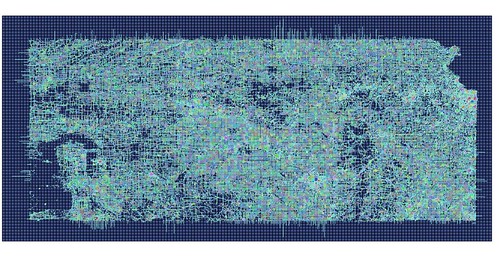All residential roads in Kansas from OSM
The background is the 3 minute interval grid used in building a graph of the roads.

I also had a quick look at Kansas (a typical mid-Western state with a gridded road system determined by township boundaries), and Oregon (mountains, a very sparsely populated interior, but lots of active mappers in the Portland & Willamette Valley areas).

I'd half expected ToeBee to have done some tidying up of highway=residential in Kansas. He's certainly tidied up lots of other things, and he knows the rural roads well as a regular participant in the annual Biking Across Kansas ride (many of his Mapillary pictures stem from these rides). The effect of a regular grid of roads, and no work to reclassify them from the original TIGER import is really obvious.


Oregon is substantially better, The local mapping community has clearly worked to improve the Tiger data along the Willamette Valley extending south from Portland. In these cases the built-up areas of local towns and cities stand out clearly. Like Pittsburgh, Portland itself is represented by several polygons divided by rivers, railways etc. Away from the centres of population we return to the 'swiss cheese; polygons. At least in some parts of the state, many of these residential roads are nothing more than forest tracks, or old farm tracks (as in the part of the John Day Fossil Beds where the family of my great-grandfather's brother ranched until around 1975). Some are, at best, vestigial.

Willamette Valley, Oregon, showing urban areas derived from residential roads.
Outlying areas can be seen to be uncorrected Tiger data, resulting in 'swiss cheese' polygons.

What this area of Oregon shows is that concerted local efforts to correct Tiger data can achieve decent results.

Remember that just the process of reviewing Tiger data can lead to substantial improvements in alignment, road detail and other things. The real problem with Tiger data is its sheer abundance, which ends up being so off-putting (and boring) that rarely do mappers stick with it. Typical rural counties in Pennsylvania have 5000 or so ways tagged highway=residential, which is a hell of a lot to review, realign, check the surface type, correct other errors, etc. The sheer amount of data involved in imports often just overwhelms the capacity of local mappers to check and enhance the imported data. This factor should always be allowed for when planning imports: if the amount of data is beyond the capacity of the community to assimilate it then it often remains untouched. Even when the data is of good quality it will get dated quite quickly.

A barn near Valencia, Butler Co, 16th July 1966

Whilst writing up this post, I've experimented with revising the classification of residential roads in Butler County, Pennsylvania. Butler is to the north of Pittsburgh, and even in the 1960s we had friends and neighbours who moved there, whilst continuing to work in the city. So although the county is still predominantly rural, there is a lot of dispersed residential settlement: either as small spur residential roads off main highways, or as non-contiguous lots along these roads. This type of settlement pattern definitely makes deciding whether residential or unclassified is the appropriate tag. One mapper has made a determined effort to map this type of landuse in a similar area just north of the Mason-Dixon Line.

View Larger Map

I focussed solely on changing tags, with a small amount of addition of a surface tag when this was really obvious. Equally, you can see, that I mainly looked at longer roads. Not only are they much easier to assess at lower zoom levels, but changing the tags of a few longer roads has a disproportionately useful effect on things like routing or my goal. I also steered clear of the larger towns which would have required more detailed examination of the aerial imagery.

Butler Co, PA: roads reassigned to unclassified.
My edits whilst writing this blog.

This approach worked fine for my goal, and should also improve things like cycle routing. Many roads are still poorly aligned, but my overall feeling is that it is more productive to concentrate on one type of change.

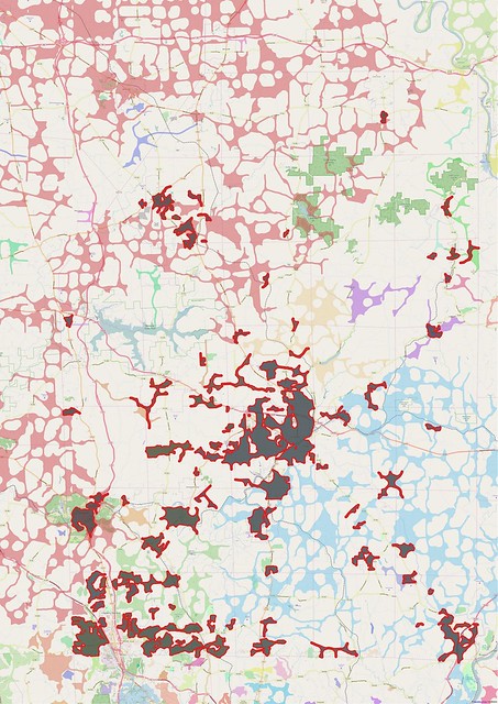Derived polygons for Butler Co, PA.
Pastel shades original polygons, grey edged with red,
derived after reclassification of rural roads (as seen aove)

The results of these changes compared to the PA dataset I started with are shown above.

Obviously for the past several years most people making use of OSM data have not been impacted by the profusion of residential roads in rural areas (and indeed in BLM lands and National Forests). Is this because most applications are agnostic to such data in the US, or is OSM data just not used in such places? The only consumer I know which does place importance on such data is Richard Fairhurst's cycle.travel, and he already makes use of landuse data to improve the quality of selected routes. It may be that highway=residential is so pervasive in the US that all data consumers have to work around this tagging, with the effect that there will be little incentive for regular mappers to change the tags.

Conclusions

This post has taken a rather meandering route.

• Firstly, the general question: "Can useful results be obtained using a very naive approach to identify urban areas?" has been answered. It works well in areas with good mapping coverage, is a decent starting points for poorly mapped places, and only falls down when tagging practices are away from the norm.

• Secondly, the data produced can provide useful visualisations which can rapidly demonstrate areas where OSM lacks data, or existing data might be better tagged.
   
• Thirdly. As for so many things with OSM, often the simplest way to work towards the data set one wants is to add more data to OSM or improve data which already exists.
• Fourthly. This approach crucially depends on availability of high quality aerial or satellite imagery for at least basic urban road networks to be mapped. Areas where only landsat data are available can never be identified with this technique.

This is not the only approach I have considered. Next up will be using OSM landuse polygons directly.

As a final note I'd like to express my particular appreciation of the work of local mappers in Pakistan, Nigeria & Cote d'Ivoire. Much of the detailed analysis and issues discussed above was based on that work.